Backpropagation is a fundamental algorithm in training neural networks. Let's break it down step by step:
反向传播是训练神经网络的基本算法。让我们一步步来解析它:
- The Neural Network Structure:
- 神经网络结构:
Imagine a simple neural network with three layers: input, hidden, and output.
想象一个简单的三层神经网络:输入层、隐藏层和输出层。
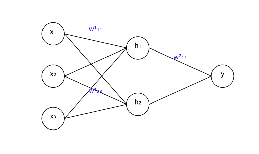
Each circle represents a neuron, and the lines represent the connections (weights) between neurons.
每个圆圈代表一个神经元,线条代表神经元之间的连接(权重)。
- Forward Propagation:
- 前向传播:
Data flows from left to right. Each neuron receives inputs, processes them, and sends an output to the next layer.
数据从左向右流动。每个神经元接收输入,处理它们,然后将输出发送到下一层。
The mathematical representation for a single neuron:
单个神经元的数学表示:
z = w₁x₁ + w₂x₂ + ... + wₙxₙ + b
a = σ(z)
Where:
其中:
- x₁, x₂, …, xₙ are inputs
- x₁, x₂, …, xₙ 是输入
- w₁, w₂, …, wₙ are weights
- w₁, w₂, …, wₙ 是权重
- b is the bias
- b 是偏置
- z is the weighted sum
- z 是加权和
- σ is the activation function (like ReLU or sigmoid)
- σ 是激活函数(如ReLU或sigmoid)
- a is the neuron's output
- a 是神经元的输出
- The Cost Function:
- 成本函数:
After forward propagation, we compare the network's output to the desired output using a cost function.
前向传播后,我们使用成本函数比较网络的输出和期望输出。
A common cost function is Mean Squared Error (MSE):
一个常见的成本函数是均方误差(MSE):
C = 1/n * Σ(y - a)²Where:
其中:
- C is the cost
- C 是成本
- n is the number of training examples
- n 是训练样本数
- y is the desired output
- y 是期望输出
- a is the network's output
- a 是网络的输出
- Backpropagation:
- 反向传播:
Now comes the crucial part. We need to figure out how each weight contributed to the error.
现在是关键部分。我们需要弄清楚每个权重如何导致误差。
We use the chain rule of calculus to calculate the partial derivatives:
我们使用微积分的链式法则来计算偏导数:
∂C/∂w = ∂C/∂a * ∂a/∂z * ∂z/∂wThis tells us how a small change in w affects C.
这告诉我们w的小变化如何影响C。
- Gradient Descent:
- 梯度下降:
Once we have these partial derivatives, we can adjust our weights:
一旦我们有了这些偏导数,我们就可以调整我们的权重:
w_new = w_old - η * ∂C/∂wWhere η (eta) is the learning rate, controlling how big our adjustment steps are.
其中η(eta)是学习率,控制我们调整步骤的大小。
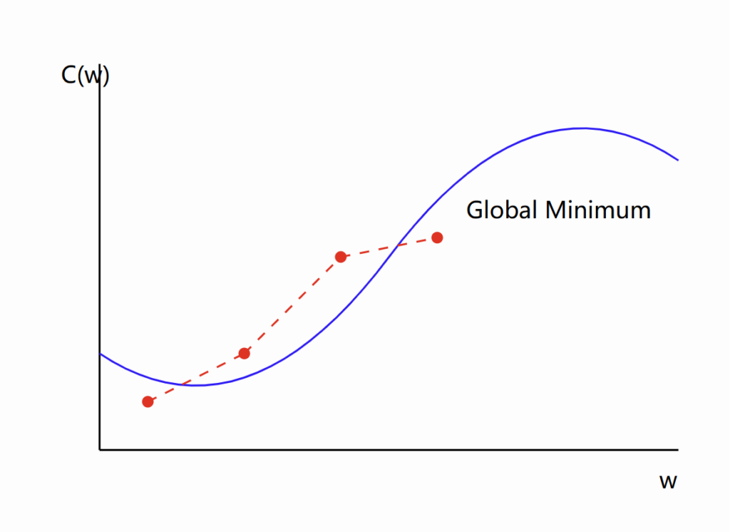
This diagram shows how gradient descent iteratively moves towards the minimum of the cost function.
这个图表显示了梯度下降如何迭代地移向成本函数的最小值。
- Iterative Process:
- 迭代过程:
Steps 2-5 are repeated many times with many training examples. This gradually improves the network's performance.
步骤2-5使用许多训练样本重复多次。这逐渐提高网络的性能。
Key Challenges:
主要挑战:
- Vanishing/Exploding Gradients: In deep networks, gradients can become very small or very large, making training difficult.
- 梯度消失/爆炸:在深层网络中,梯度可能变得非常小或非常大,使训练变得困难。
- Local Minima: Gradient descent might get stuck in a local minimum instead of finding the global minimum.
- 局部最小值:梯度下降可能陷入局部最小值,而不是找到全局最小值。
Advanced Techniques:
高级技术:
- Momentum: Adds a fraction of the previous weight update to the current one, helping to overcome local minima.
- 动量:将前一次权重更新的一部分添加到当前更新,有助于克服局部最小值。
- Adam Optimizer: Adapts the learning rate for each weight, often leading to faster convergence.
- Adam优化器:为每个权重自适应学习率,通常导致更快的收敛。
- Batch Normalization: Normalizes the inputs to each layer, which can speed up learning and reduce the dependence on careful weight initialization.
- 批量归一化:归一化每层的输入,可以加速学习并减少对仔细权重初始化的依赖。
Understanding backpropagation is crucial for anyone working with neural networks. While the math can be complex, the core idea is simple: learn from mistakes and make small, calculated improvements over time.
理解反向传播对于任何使用神经网络的人来说都是至关重要的。虽然数学可能很复杂,但核心思想很简单:从错误中学习,并随着时间的推移做出小的、经过计算的改进。
For further exploration:
进一步探索:
- "Neural Networks and Deep Learning" by Michael Nielsen: An in-depth, free online book.
- Michael Nielsen的"神经网络与深度学习":一本深入的免费在线书籍。
- TensorFlow Playground: An interactive visualization of neural networks.
- TensorFlow Playground:神经网络的交互式可视化。
- CS231n: Convolutional Neural Networks for Visual Recognition - Stanford University course materials.
- CS231n:用于视觉识别的卷积神经网络 - 斯坦福大学课程材料。
Remember, mastering these concepts takes time and practice. Don't be discouraged if it doesn't all make sense immediately!
记住,掌握这些概念需要时间和练习。如果不能立即理解所有内容,不要灰心!